Gradient descent approximation
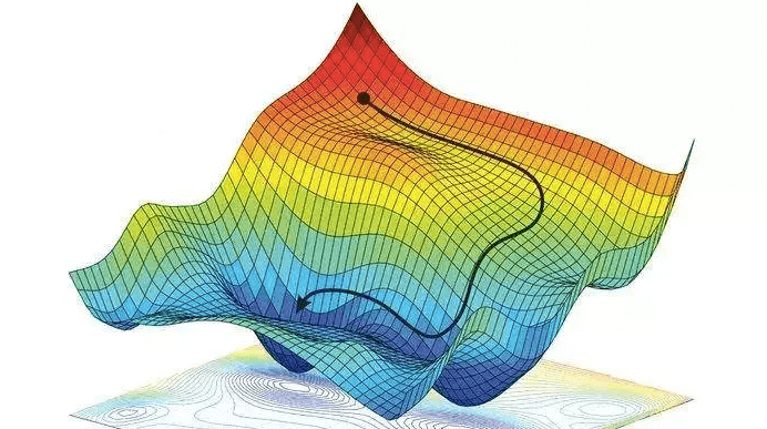
A linear regression model attempts to explain the relationship between a dependent (output variables) variable and one or more independent (predictor variable) variables using a straight line.
This straight line is represented using the following formula: y = mx +c
Where, y: dependent variable
x: independent variable
m: Slope of the line (For a unit increase in the quantity of X, Y increases by m.1 = m units.)
c: y intercept (The value of Y is c when the value of X is 0)
The first step in finding a linear regression equation is to determine if there is a relationship between the two variables. We can do this by using the Correlation coefficient and scatter plot. When a correlation coefficient shows that data is likely to be able to predict future outcomes and a scatter plot of the data appears to form a straight line, we can use simple linear regression to find a predictive function. Let us consider an example.
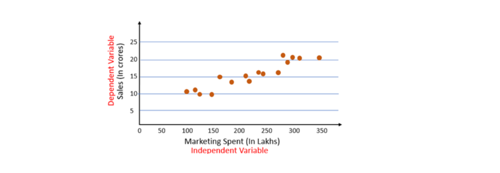
From the scatter plot we can see there is a linear relationship between Sales and marketing spent. The next step is to find a straight line between Sales and Marketing that explain the relationship between them. But there can be multiple lines that can pass through these points.

So how do we know which of these lines is the best fit line? That’s the problem that we will solve in this article. For this, we will first look at the cost function.
Cost Function
The cost is the error in our predicted value. We will use the Mean Squared Error function to calculate the cost.
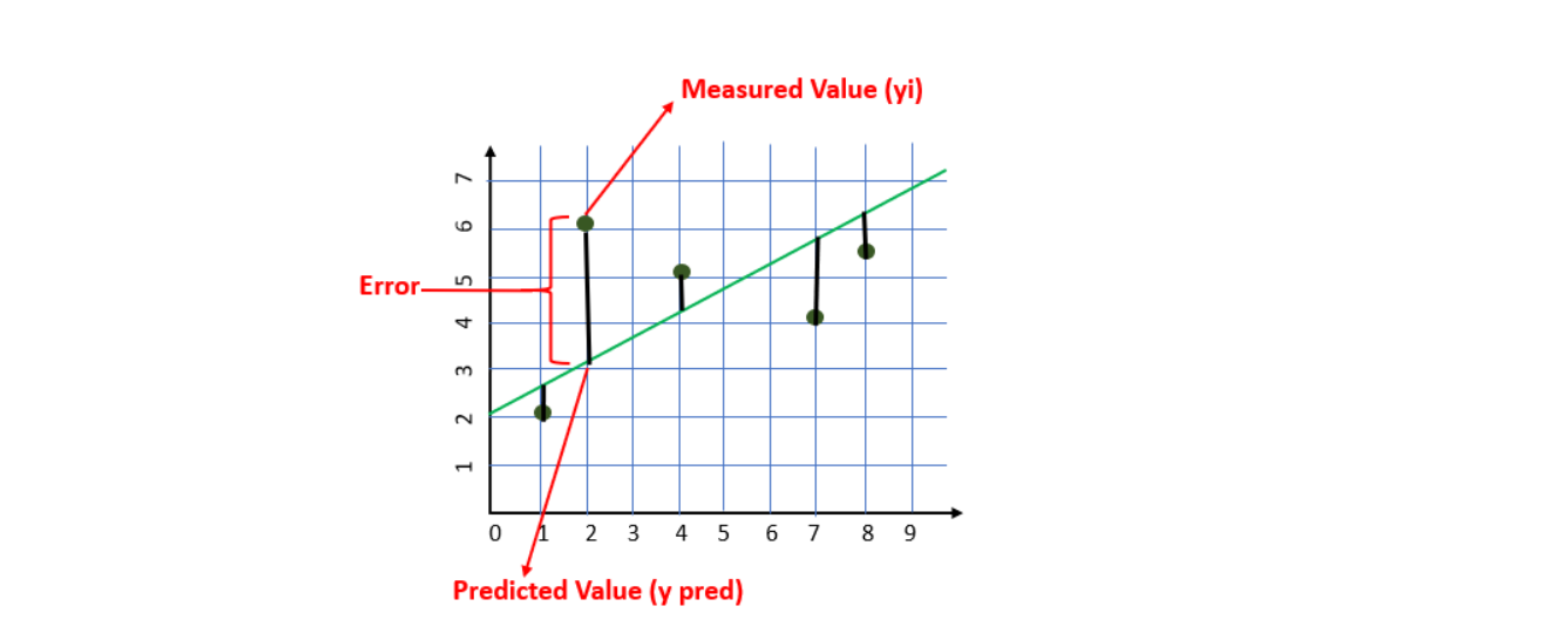

Our goal is to minimize the cost as much as possible in order to find the best fit line. We are not going to try all the permutation and combination of m and c (inefficient way) to find the best-fit line. For that, we will use Gradient Descent Algorithm.
Gradient Descent Algorithm
Gradient Descent is an algorithm that finds the best-fit line for a given training dataset in a smaller number of iterations. If we plot m and c against MSE, it will acquire a bowl shape (As shown in the diagram below)
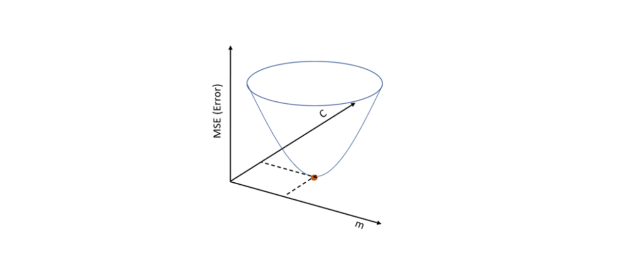
For some combination of m and c, we will get the least Error (MSE). That combination of m and c will give us our best fit line.
The algorithm starts with some value of m and c (usually starts with m=0, c=0). We calculate MSE (cost) at point m=0, c=0. Let say the MSE (cost) at m=0, c=0 is 100. Then we reduce the value of m and c by some amount (Learning Step). We will notice a decrease in MSE (cost). We will continue doing the same until our loss function is a very small value or ideally 0 (which means 0 error or 100% accuracy).
Step by Step Algorithm:
Step 1: Let m = 0 and c = 0. Let L be our learning rate. It could be a small value like 0.01 for good accuracy.
Learning rate gives the rate of speed where the gradient moves during gradient descent. Setting it too high
would make your path instable, too low would make convergence slow. Put it to zero means your model
isn’t learning anything from the gradients.
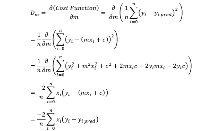
Step 2: Calculate the partial derivative of the Cost function with respect to m. Let partial derivative of the
Cost function with respect to m be Dm (With little change in m how much Cost function changes).
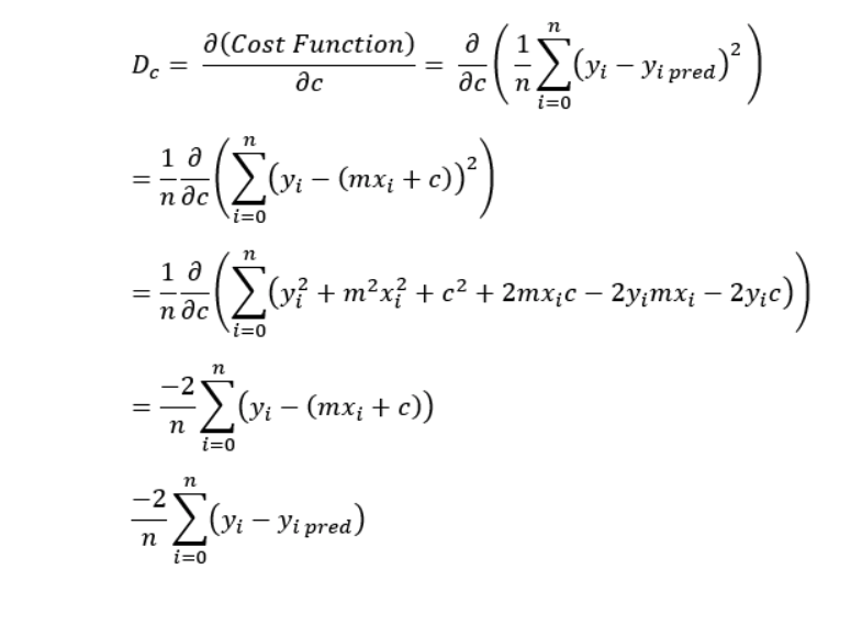
Similarly, let’s find the partial derivative with respect to c. Let partial derivative of the Cost function with respect to c be Dc (With little change in c how much Cost function changes).
3. Now update the current values of m and c using the following equation:

4. We will repeat this process until our Cost function is very small (ideally 0).
Gradient Descent Algorithm gives optimum values of m and c of the linear regression equation.
With these values of m and c, we will get the equation of the best-fit line and ready to make predictions.
References
All credit goes to: https://www.analyticsvidhya.com/blog/2021/04/gradient-descent-in-linear-regression/