Types of optimizers
This blog post aims at explaining the behavior of different algorithms for optimizing gradient parameters that will help you put them into use.
In this post we will learn about
1. Batch Gradient Descent
2. Stochastic Gradient Descent
3. Mini-batch Gradient Descent
4. Adagrad
5. RMSprop (similar to Adadelta but uses RMS)
6. Adam
All of these tries to lower the loss function by updating the model parameters in response to the output of the loss function. Thereby helping to reach the Global Minima with the lowest loss and most accurate output.
Important function of the optimizer is to update the weights of the learning algorithm to reach the least cost function. Here is the formula used by all the optimizers for updating the weights with a certain value of the learning rate.

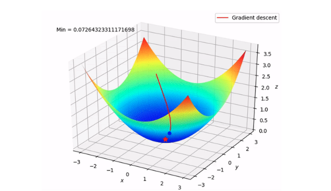
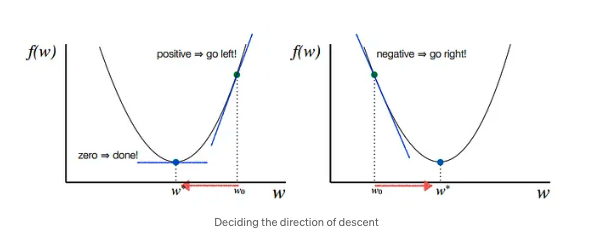
1. Gradient Descent
This optimizer used in neural networks, best for the cases where the data is arranged in a way that it possesses a convex optimization problem. It will try to find the least cost function value by updating the weights of your learning algorithm and will come up with the best-suited parameter values corresponding to the Global Minima.
This is done by moving down the hill with a negative slope, increasing the older weight, and positive slope reducing the older weight.
Although there are challenges while using this optimizer, suppose the data is arranged in a way that it possesses a non-convex optimization problem then it can possibly land on the Local Minima instead of the Global Minima thereby providing the parameter values with a higher cost function.
There is also a saddle point problem. This is a point where the gradient is zero but is not an optimal point. This is still an active area of research.
For certain cases, problems like Vanishing Gradient or Exploding Gradient may also occur due to incorrect parameter initialization. These problems occur due to a very small or very large gradient, which makes it difficult for the algorithm to converge.
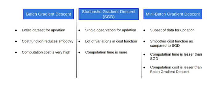
Let’s say there are a total of ‘m’ observations in a data set and we use all these observations to calculate the cost function J, then this is known as Batch Gradient Descent.
2. Stochastic Gradient Descent
This is another variant of the Gradient Descent optimizer with an additional capability of working with the data with a non-convex optimization problem. The problem with such data is that the cost function results to rest at the local minima which are not suitable for your learning algorithm.
Rather than going for batch processing, this optimizer focuses on performing one update at a time. It is therefore usually much faster, also the cost function minimizes after each iteration (EPOCH). It performs frequent updates with a high variance that causes the objective function(cost function) to fluctuate heavily. Due to which it makes the gradient to jump to a potential Global Minima.
However, if we choose a learning rate that is too small, it may lead to very slow convergence, while a larger learning rate can make it difficult to converge and cause the cost function to fluctuate around the minimum or even to diverge away from the global minima.
If you use a single observation to calculate the cost function it is known as Stochastic Gradient Descent, commonly abbreviated as SGD. We pass a single observation at a time, calculate the cost and update the parameters.
3. Mini-batch Gradient Descent
Another type of Gradient Descent is the Mini-batch Gradient Descent. It takes a subset of the entire dataset to calculate the cost function. So if there are ‘m’ observations then the number of observations in each subset or mini-batches will be more than 1 and less than ‘m’.
4. Adagrad
This is the Adaptive Gradient optimization algorithm, where the learning rate plays an important role in determining the updated parameter values. Unlike Stochastic Gradient descent, this optimizer uses a different learning rate for each iteration(EPOCH) rather than using the same learning rate for determining all the parameters.
Thus it performs smaller updates(lower learning rates) for the weights corresponding to the high-frequency features and bigger updates(higher learning rates) for the weights corresponding to the low-frequency features, which in turn helps in better performance with higher accuracy. Adagrad is well-suited for dealing with sparse data.
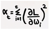
So at each iteration, first the alpha at time t will be calculated and as the iterations increase the value of t increases, and thus alpha t will start increasing.
Now the learning rate is calculated at each time step. Given by,
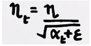
Here epsilon is a small positive number added to alpha to avoid the error if at any instance alpha becomes zero
However, there is a disadvantage of getting into the problem of Vanishing Gradient because after a lot of iterations the alpha value becomes very large making the learning rate very small leading to no change between the new and the old weight. This in turn causes the learning rate to shrink and eventually become very small, where the algorithm is not able to acquire any further knowledge.
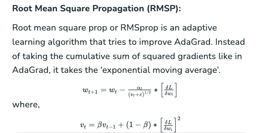
5. RMSprop
This is an extension of the Adaptive Gradient optimizer, taking care of its aggressive nature of reducing the learning rate infinitesimally. Here instead of using the previous squared gradients, it takes the ‘exponential moving average’ of all past squared gradients.
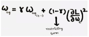
At each iteration, first the weighted average is calculated. Where we have the restricting term(gamma = 0.95) which helps in avoiding the problem of Vanishing Gradient.
After which the Learning rate is calculated using the formula,
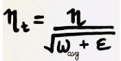
Thus because of the restricting term, the weighted average will increase at a slower rate, making the learning rate to reduce slowly to reach the global minima.
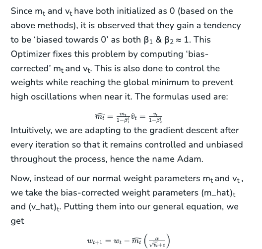
6. Adam
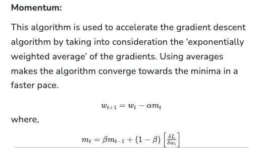
This is the Adaptive Moment Estimation algorithm which also works on the method of computing adaptive learning rates for each parameter at every iteration. It uses a combination of Gradient Descent with Momentum and RMSprop to determine the parameter values.
Adam optimizer involves a combination of two gradient descent methodologies: